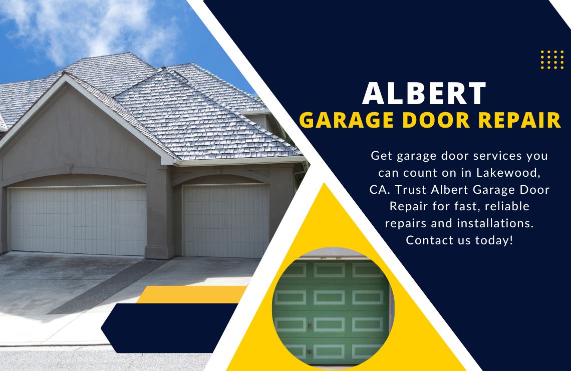
Welcome to Albert Garage Door Repair, your premier destination for top-notch garage door services in Lakewood, CA. Our expert technicians are dedicated to providing fast, reliable repairs and installations that will keep your garage door running smoothly and efficiently.Whether you're dealing with a broken spring or need a brand new installation, we've got you covered.
(562) 837-2794At Albert Garage Door Repair, we offer a wide range of expert garage door services in Lakewood, CA, including installation, maintenance, and repair to ensure that your garage door is functioning smoothly and efficiently.
By choosing Albert Garage Door Repair's professional services, you'll enjoy improved safety and security, longer lifespan of your garage door, and expert advice on maintenance.
Professional garage door repair services can significantly improve the
safety and security of your home. A malfunctioning or damaged garage
door can pose a significant threat to your family's safety, as it could
fall unexpectedly or fail to open properly.
Additionally, an unreliable garage door is a potential entry point for
burglars and intruders. Professional technicians from Albert Garage Door
Repair in Lakewood CA have the experience and expertise necessary to
ensure that your garage door operates safely and securely.
Moreover, professional maintenance services such as regular lubrication
of moving parts, adjustment of springs and hinges, and inspection of
electrical components can help prevent unexpected malfunctions that may
cause injuries or property damage.
Having a functional garage door can add to the convenience of your daily
routine. Imagine being able to effortlessly park your car in the garage
without having to struggle with a faulty door that won't open or close
properly.
By choosing Albert Garage Door Repair for your garage repair needs, you
can enjoy increased convenience as our skilled technicians work quickly
and efficiently to fix any issues you may be experiencing.
Whether it's a broken spring, faulty opener, or off-track door, we will have your garage door running smoothly again in no time.